Seven areas · Select a tile to explore its charts.
Favourable trendMixed pressuresHigh pressure
Counts include dedicated and shared charts; a shared chart appears in each relevant area. Editorial assessments · reviewed 17 October 2026. Colours combine direction and consequences; they are not automatic risk scores or labels for how fast a curve grows.
Why these colours? Read the evidence and limits
01 / ACCELERATING WORLD - MONITORING SEVEN AREAS
Every indicator. Room to see the whole curve.
Sixteen indicator cards with 20 main graph panels, plus recovery details and thematic and scenario explorers. Each panel has its own dates, time window and trend context.
10 years, 50 years and All available count back from each panel’s latest historical year. The urbanisation panel adds a labelled 2026 projection to its historical window; the waste panel counts back from 2026, including labelled projections. Trend tags and historical CAGR tiles keep their stated reference periods. Open “Explore” for further analysis, source notes and data downloads.
02 / PEOPLE & DISTRIBUTION
Growth for whom? Concentrated where?
Average progress can hide different experiences. Distribution, ageing and the geography of growth belong beside the headline totals.
DISTRIBUTION
Who holds the wealth?
Compare the top tenth with the bottom half. Start with wealth, or switch to income for a different view of inequality. The world view and the distribution within a country answer different questions.
WID estimates, equal-split adults. Income is pre-tax national income after pensions; wealth is net personal wealth. Current downloaded histories end in 2023. They are not the separate 2025 snapshots in WIR 2026.
Not necessarily. A city can grow outward while its population grows. Compare population, people per square kilometre and concentration in a country's cities.
Six illustrative cities, not a representative global sample. UN WUP 2025 uses harmonised DEGURBA settlement extents, not administrative boundaries. Density is not a direct measure of crowding or service quality.
UN World Population Prospects 2024, processed by Our World in Data. Estimates end in 2023; 2024 onward, including 2026, is a medium-variant projection. Dashed lines are projections, not observed outcomes. Source ↗
03 / THE COMING OF AI
A new capacity to act. A new question of control.
AI connects the trends above: computation and data become tools that can help people analyse, create and act. The question is how to turn expanding capability into useful, widely shared progress.
MEASURING CAPABILITY
What has changed?
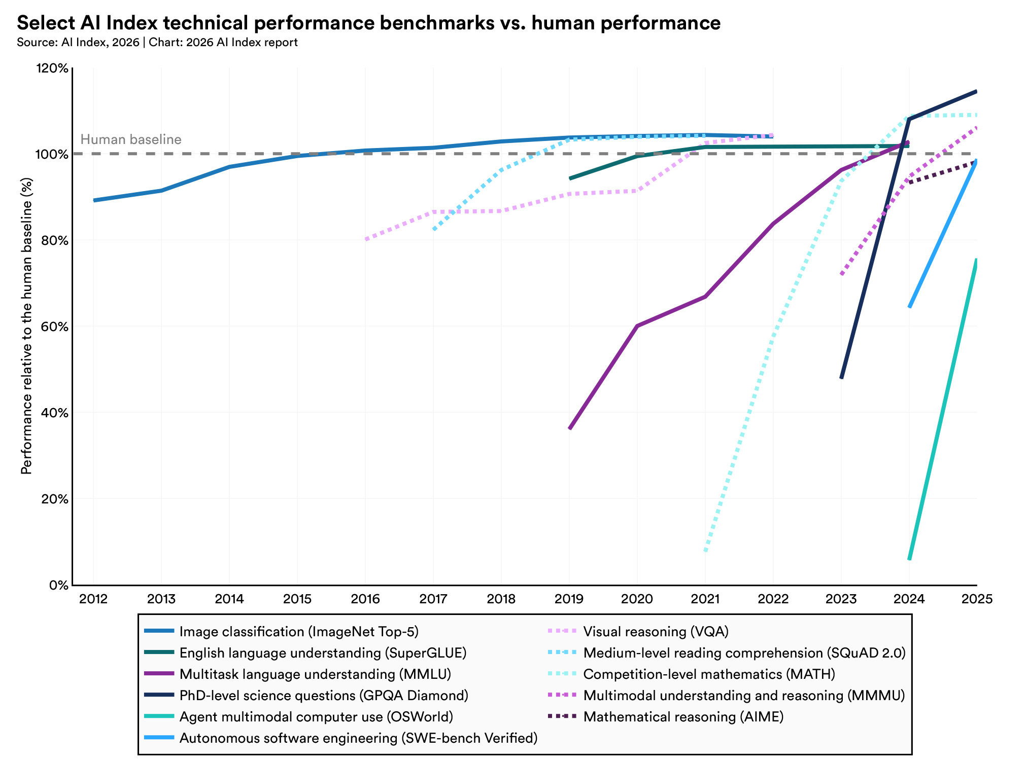
Selected tests show rapid gains in language, scientific questions, coding and computer use. Several cross their human reference level; others remain below it. These are different tasks, not one measure of intelligence.
Stanford HAI, AI Index 2026, Figure 2.1.1 · data through 2025. Each line has its own human reference; 100% is not perfect accuracy. Different systems can supply the results across tasks and years. Tap the chart to enlarge.
A higher benchmark score opens possibilities. Dependable performance outside the test requires separate evidence.
Benchmarks can saturate, contain errors or reward familiarity with a test. Read this as evidence of changing task capability, not proof of general judgment or safe autonomy. Source and interpretation ↗
WHY NOW?
Three advances reinforce one another.
Better data
Useful examples, careful selection and checked demonstrations shape what a model can learn. Quality and coverage matter alongside volume.
Better learning methods
Architectures, training objectives and feedback change how a model uses its examples. Pre-training builds broad patterns; post-training shapes behaviour and task performance.
Better computation
Accelerators, memory and parallel processing make larger training runs and more experiments feasible. Efficient software helps turn hardware into useful work.
Better examples improve learning; better methods use resources more effectively; more usable computation expands what can be tried.
Conceptual explanation, not a measured allocation of progress between three causes.
From microprocessors to AI chips
The transistor curve spans more than half a century. Moore’s roughly two-year doubling became an industry reference, not a law guaranteeing performance. Modern GPUs add parallel computation and advanced packaging; some combine multiple compute dies. Transistor totals therefore do not measure speed, efficiency or useful work on their own.
Memory, data movement, numerical precision and software also matter. The same hardware can deliver different results depending on how it is used.
Stanford’s 2025 AI Index reports that the price of querying a model at a fixed GPT-3.5-level benchmark threshold fell from $20 to $0.07 per million tokens between November 2022 and October 2024—more than a 280-fold reduction. This compares a particular performance threshold, not every model or the full cost of deploying AI.
Lower prices can widen access. Useful adoption still depends on skills, reliable infrastructure, suitable workflows and who controls the tools.
Agents could coordinate longer workflows across software. The test is successful completion with bounded permissions, clear accountability and a way to stop or undo actions.
From analysis to discovery
AI could help propose molecules, materials and experiments. The test is independently validated results, useful treatments and wider access—not simply more generated candidates.
From screens to the physical world
Robotics could extend assistance into factories, care and daily life. The test is reliable operation in varied environments, at an acceptable cost and level of risk.
These are possible paths and proposed tests of progress. Their speed and reach remain uncertain; no date for general intelligence is implied.
How AI could affect all seven areas
Illustrative opportunities and pressures to examine, not measured net effects.
Area
Potential contribution
Question of control
Population
Care assistance and planning for changing needs
Does support preserve autonomy and reach underserved communities?
Economy
Productivity and new services
Who gains, who is displaced, and how concentrated are the returns?
Technology
Faster design, coding and experimentation
Can testing and oversight keep pace with deployment?
Data
Better analysis and cyber defence
How do we limit surveillance, misuse and automated attacks?
Environment
Resource optimisation and environmental monitoring
Do verified savings exceed added energy and material demands?
Health
Research and clinical assistance
Are benefits validated, affordable and reliable across populations?
Freedom & society
Access to knowledge and participation
Can people challenge decisions and retain independent judgment?
Faster capability is not the objective by itself.
AI could increase the pace of change and improve our ability to respond. Which effect dominates depends on deployment, institutions and the distribution of power. The aim is a sustainable pace of useful progress, with the capacity to detect harm, correct mistakes and share the gains.
Acceleration and absorption. From growth to the capacity to respond.
The shape of a curve changes the demands a system must absorb. Compounding, connectedness and cycles help explain those demands; our ability to observe, act and correct determines how well we respond.
SCHEMATIC CURVES · NOT FORECASTS
Three curves, three different stories.
A rising level is not enough to establish an increasing percentage growth rate. Read the shape, the time horizon and what is growing.
Linear
Equal absolute additions. The level rises, while percentage growth declines.
Exponential
A constant percentage applied to a growing base. Absolute additions become larger.
Saturation / S-curve
Growth first gathers pace, then slows towards a limit. Stabilisation is a possibility, not a universal outcome.
Illustrative shapes on a shared linear index scale, starting at 1. Time is schematic; these are not fitted histories.
01 / COMPOUNDING
Growth builds on growth.
Each increase expands the base for the next. Several drivers can also reinforce one another. A small sustained rate can create a large change in scale.
02 / CONNECTEDNESS
Consequences cross domains.
A change in one area can alter demands in another: more data can require more energy and stronger security. Interactions may amplify or dampen pressure.
03 / CYCLICITY
Trajectories can turn.
Feedback, constraints and recurring cycles can interrupt expansion or bring reversal. Neither endless growth nor inevitable collapse follows from a rising curve alone.
ARITHMETIC ILLUSTRATION
What a century does to a small percentage.
Every line starts at 1. The annual percentage stays constant; the amount added each year grows.
All four rates
Lower rates, closer view
Linear axes in both panels, with different vertical ranges. Level = (1 + annual rate)years. Constant rates, no shocks or saturation: mathematical scenarios, not forecasts. Multipliers show the level reached, not the sum of annual flows.
What grows matters.
If the rising quantity is an annual physical burden, each year can demand more collection, treatment or infrastructure. Unresolved flows can accumulate into a stock even when their growth slows. Capacity, prevention and ecological limits determine the consequences.
FROM SCALE TO RESPONSE
Can the capacity to respond keep pace?
Absorption means the practical ability to handle change: understand it, act on it and correct its consequences. A one-time improvement can create breathing room, but sustained growth may use it up. The following scenario compares pressure and response on one assumed scale; it does not claim a measured global absorption limit.
ILLUSTRATIVE SCENARIO · CYBERSECURITY
A one-time capacity gain buys time. It does not stop workload growth.
Common workload index: manual capacity = 100. All future lines are assumptions, not observed global cyber threats or a forecast of attacks.
What comes from evidence, and what is assumed?
This example uses a Microsoft October 2025 randomised study of 167 professional analysts. Its workflow calculations imply roughly 3.1–6.5× correctly identified malicious emails per analyst-minute under particular prevalence, precision and recall assumptions. The lower 3.1× case assumes 20% malicious mail and 80% precision and recall, with automated benign-mail handling.
The 20% annual workload increase is illustrative. Staffing, task mix and effectiveness are held constant; implementation overhead, errors and automation bias are not modelled. A task-specific vendor study does not establish a 3.1× reduction in breaches or a universal productivity gain.
Measure detection delay, error rates and the human ability to check an answer. Faster output alone does not establish better judgment.
02
Decide & respond
Measure the time from a warning to action, trained staff and available infrastructure. Capacity is specific to the task.
03
Correct & recover
Measure appeal times, fallback readiness and successful recovery. A response system needs a practical way to change course.
Control can enable useful speed. Explore how prevention, greater response capacity and shorter delays change the gap in Pace and Control Simulator ↓.
05 / PACE AND CONTROL SIMULATOR
Pace and Control Simulator. Choose the pace. Build the response.
Explore the conceptual relationship between pressure, adaptive capacity and exposure. These controls express assumptions; they do not measure the world's current state.
Acceleration potential A
Adaptive capacity C
Relative pressure Ω
A = ∛(P × I × N) C = ∛(G × R × L) Ω = (A ÷ C) × E
Dimensionless conceptual ratios, not calibrated indicators, probabilities or safety thresholds. The time paths are an illustrative extension: pressure = 100 × A × E × (1 + p)t; capacity = 100 × C × (1 + c)max(0, t − delay). Equal values only mean equality on this assumed common scale. No empirical global “absorption capacity” is claimed.
SOURCE ESTIMATES
The recovery gap.
Electronic waste generation and documented formal collection and recycling, in million tonnes per year.
48.2 Mt / year
Generation minus documented formal recovery, 2022 Up from 26 Mt in 2010
Formal recovery is a measurable response, not total societal absorption. The remainder includes informal recycling, storage and other destinations; it is not all landfill or proven harm.
A model can reveal a gap. Institutions need the authority, knowledge and accountability to act on it. These possible structures are proposals for discussion, not a claim that one design fits every society.
Control with checks, participation and correction.
AI can help detect risks, compare options and evaluate results. Decisions affecting rights, public resources and acceptable risks need accountable human authority. No single operator should both make consequential decisions and be the sole judge of their effects.
OPTION A / PUBLIC AUTHORITY
Democratic mandate. Independent scrutiny.
Elected institutions set objectives and limits. A competent public authority supervises implementation, while independent auditors and courts provide scrutiny and avenues for remedy.
Strength and vulnerability
A clear mandate and enforcement powers can support action. Political capture, slow procedures and limited technical capacity can weaken oversight. Published reasons, conflict-of-interest rules and periodic review are essential safeguards.
OPTION B / SHARED OVERSIGHT
Bring affected people into the decision.
A public-interest council brings together citizens, domain experts, workers, operators and public authorities. It examines trade-offs and recommends conditions; a named accountable authority retains responsibility for binding decisions.
Strength and vulnerability
Broader participation can reveal overlooked harms and priorities. Unequal resources and unclear responsibilities can distort deliberation. Balanced representation, transparent selection and clear decision rights help address these weaknesses.
OPTION C / COORDINATED LEVELS
Local action. Shared safeguards.
Local and sector bodies handle decisions close to those affected. National institutions set minimum protections and hear escalations. International cooperation addresses impacts that cross borders.
Strength and vulnerability
Decisions can reflect local conditions while sharing knowledge. Gaps between jurisdictions and fragmented enforcement remain risks. Common reporting, explicit escalation routes and coordination agreements help connect the levels.
A correction process for any structure.
These structures can be combined. Each needs a visible route from evidence to action, and from a contested decision to a remedy.
Observe & disclosePublish indicators, incidents, uncertainties and who is responsible. Protect privacy and legitimate confidential information.
Deliberate & decideHear affected groups, compare alternatives and record reasons, limits and review dates.
Act & evaluateUse bounded implementation, monitor outcomes and check whether benefits and burdens are fairly distributed.
Challenge & appealGive affected people an accessible way to request an explanation, independent review and correction or reversal.
Pause, repair & reviewDefine emergency triggers and who may pause a system. Provide safe fallback, time-limited powers, independent review and conditions for restart.
Appeals need published response deadlines and protection against retaliation. Emergency intervention must be proportionate: stopping a critical service can itself cause harm. Review findings should feed back into the next decision.
Measure whether control works.
Track time from warning to action, access to appeals, correction and recovery times, recurrence of failures, distribution of impacts and concentration of decision power. Assess these together: a fast decision is not necessarily a good one, and a low appeal count may reflect barriers to challenge.